Make Data Easy To Analyze With Conditional Formatting in SpreadProcessing

Let’s get an overview of the new Conditional Formatting functionality in SpreadProcessing.

With the latest R1 2022, we introduced two of the most-demanded features in our SpreadProcessing library—Notes and Conditional Formatting. Today I would like to show you a brief overview of the conditional formatting support and how you can use this feature with SpreadProcessing.

What Is Conditional Formatting?

Conditional formatting comes as great help when you need to apply styling on cells according to the data they contain. With this functionality, you can ensure that the data will be always easy to read and the end users will be able to focus on important points inside. Furthermore, the styling of the cells will dynamically change if that is needed when the value of a cell is modified.

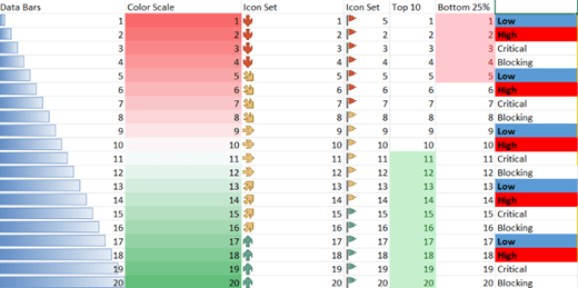
You can apply various formatting options like changing fill and font and even create more complex rules with data bars, color scales and icon sets. You can see some examples in the screenshot below.

To give you a better understanding of the API SpreadProcessing exposes, let’s first take a look of the building elements of the conditional formatting:

• Rule – defines the condition that the values should be evaluated against. If the condition is evaluated to a value bigger than 0, the cell range is formatted; otherwise, if the condition results in 0, the cell range is not formatted.
• Formatting – defines the formatting that should be applied to all the cells whose value falls within the condition constraints.

There is an extensive set of predefined rules that you can use in SpreadProcessing and creating custom ones through formulas is also supported. Since I don’t want to bore you with long lists, if you are eager to check all of the built-in rules, they are available in the dedicated Conditional Formatting help topic.

Conditional Formatting in Action

After introducing you the basics of the feature, I suggest it’s time to look at some examples of how it works.

Let’s assume that you are keeping an eye on some companies you bought shares from. With the conditional formatting, you can easily find the companies that are not profitable enough or such that can bring you more earnings. Here is the data we have:

There are several things we can make to better visualize this data and make it easy to read and make decisions from. The first one is to highlight the distribution of the shares so you can immediately see which are the companies you bought mostly from. This can be done using the DataBar rule:

Now you can see the distribution of the shares from the first sight:

Anyone would be also interested in the investments that turn out to be dropping on yearly basis. Let’s emphasize on them using the Formula rule. When using this rule, the cell values that evaluate to true will be highlighted by the rule formatting. The specific formula used in the snippet below will pick up all the shares whose price has decreased, or the increase is with less than $10.

Now you can see which shares are dangerous for your savings.

The Change column can help you even more to make the most appropriate decision. I would suggest adding icons to it that show how the shares perform:

I believe you will agree with me that it is a matter of seconds to notice which shares would be better to get out of your portfolio and which one you should be keeping an eye on.

Of course, this is a pretty simple example showing a small part of all the fancy formattings you can apply and the rules you can use for them. I am sure that you are dealing with much more diverse data and there are many points of improving its visualization. Thus, don’t wait to surprise your customers with new shiny documents.

Try It and Share Your Feedback

No matter if you are already familiar with Telerik Document Processing or will meet the libraries for the first time, hurry up and get the latest bits so you can explore all the possibilities they provide:

Download a Free Trial

And I am sure I have told you many times that your input is valuable. We do listen. So, do not be shy—drop us a line to share your feedback in the comments section below or directly in our Document Processing Libraries Feedback Portal.

Happy formatting!